Introduction and Motivation

Type 2 diabetes is a serious medical condition affecting over 30 million Americans and approximately 9 in 110 people worldwide (Zheng). Type 2 diabetes is not an isolated condition, and it is often preceded by dietary and/ or overall health concerns. The Pima Indians are a Native American tribe living in Arizona, and their genetic traits have predisposed them to survival on a low-carb diet. Within the past 100 years, the Pima’s have developed the highest prevalence of Type 2 diabetes in the world, making them of much interest to researchers.

In this project, we seek to compare the performance of many classical machine learning algorithms and models by testing them on the classification problem associated with whether a given person has diabetes or not. Additionally, we would like to isolate what features correlate with each other at a higher degree with a diabetes diagnosis.

Using Kmeans and other visualization techniques, we would like to observe the correlations and distribution of features that lead to a diagnosis of diabetes. We expect that high glucose, BMI and low insulin levels will have a strong correlation with the diagnosis of diabetes given the generally known nature of the diseases (Balkau). However, we expect that age will be uncorrelated with diabetes while high blood pressure and diabetes will have a positive correlation. Additionally, we believe it would be interesting to look at the correlation between genetic factors described by the Pedigree Factor of subjects vs environmental factors such as glucose and BMI.

Dataset

Features

The dataset contains eight total features: Pregnancies, Glucose Level (mmol/L), Blood Pressure (mmHg), Skin Thickness (mm), Insulin (muU/ml), BMI (kg / height in meters squared), Diabetes Pedigree Function, and Age (years). The outcome is binary with 768 total outcomes; 268 are 1 and the rest are 0. The dataset was adapted from the National Institute of Diabetes and Digestive and Kidney Diseases, specifically from females twenty-one or older of Pima Indian heritage. The dataset was retrieved from the UCI Machine Learning Repository. One interesting point is that there are far greater outcomes with diabetes than without.

Data Cleaning

The dataset did have some missing values. For example: BMI, Blood Pressure, Glucose, and Skin Thickness were 0 for a large number of data points. Medically speaking having 0 for these features does not make sense. Therefore to handle this missing/invalid data, we replace those values with the median for the feature. Since the features had different ranges and scales, we also standardized the data, so no one feature dominates.

Distribution of data

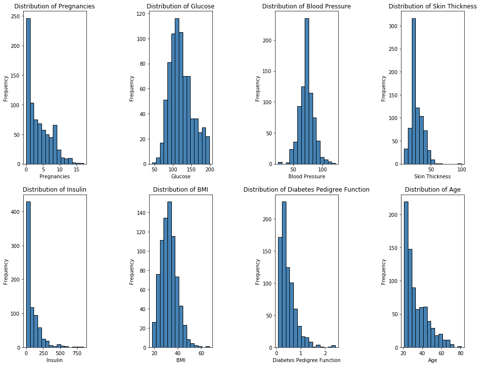
Shown below are Histograms of our 8 features. One important observation is that half of our features, Pregnancies, Age, Insulin, and Diabetes Pedigree Function, are not normally distributed, instead they are right skewed, while the other half is relatively normally distributed.

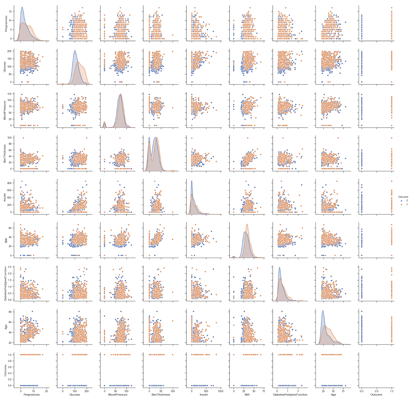
Looking at the visualization of the data set below we can see that many of the features do not give us a clear separation between having diabetes and not. However there slightly greater separation in the plots where glucose forms the x-axis between the outcome of having diabetes vs the outcome of not having diabetes. Although it may be obvious that a higher level of glucose indicates the presence of diabetes due to general assumptions we all have heard about the disease it is clear from this that it is strongly isolated from normal glucose levels and thus higher glucose levels in combination with other features may provide more information.

Feature Correlation

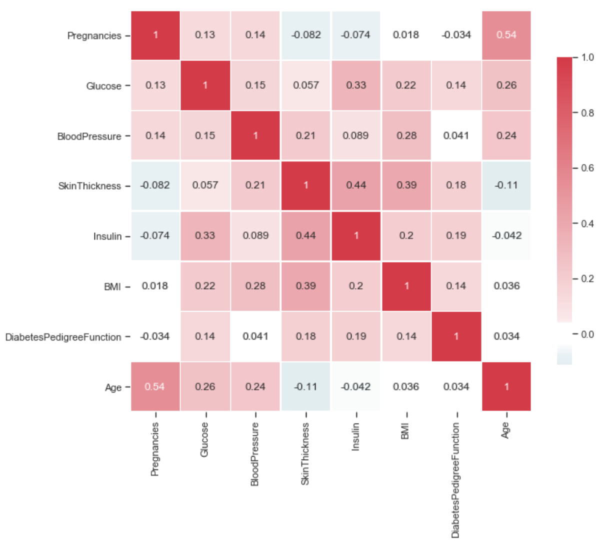Feature Correlation provides us with information about how each feature is related to each other. The lower the value or lower the color, the less correlated they are. The opposite stands true for the case when we have the case where the color is darker or have a larger value.

Approach

For the purposes of classification, we would like to compare the performance of many common supervised models including Random Forest, SVM, and Logistic Regression. In addition to the above, we would also like to test clustering models, specifically K-means and GMM. We plan to run the models as if the labels do not exist and compare this to the actual labels of the data. Based on research and known previous efforts with this type of prediction, we hope to achieve a minimum of 70% accuracy.

Unsupervised Learning

We implemented the following unsupervised algorithms as if our dataset did not possess labels with the intent of comparing the computed labels to the actual labels for measuring accuracy.

Kmeans

Although our dataset is labeled, we were interested in knowing how accurately K-means would cluster the data vs our ground truth labels given in the data set when ran with the optimal number of clusters. This would imply that people with/without diabetes are located close spatially.

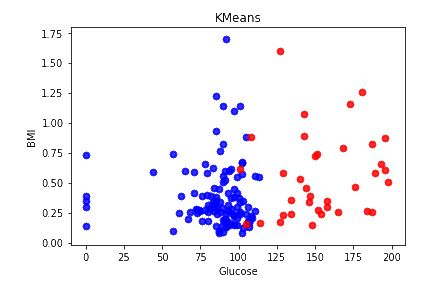
KMeans accuracy: 0.66015625

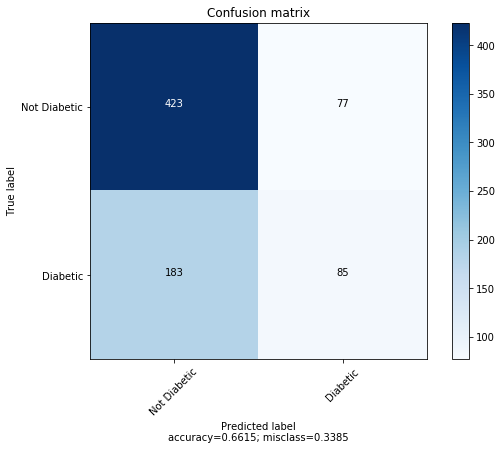
This is only slightly better than guessing “no diabetes” on every datapoint.

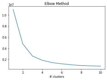
While the actual number of clusters is 2, using the elbow method we can see that the optimal number of clusters for Kmeans is 3 or 4. This indicates that the data is not split into two clusters, have diabetes vs does not have diabetes.

As noted in our initial observations of the data set, there really are no clear separations between the features when looking at the pair plots. We can only find one feature that is slightly separated, i.e. glucose. This lack of spatial separation greatly affects the accuracy of K-means as it relies on a distance function.

GMM

GMM utilizes different Gaussian distribution to provide a soft-mapping into each cluster, in contrast, K-means relies on hard-mapping. This may have contributed to GMMs terrible accuracy. By soft clustering on relatively overlapping data, the two clusters converge and points near each other and all points have relatively high likelihood of being in both clusters. In other words, it would have a 50/50 chance of being in either cluster. In addition, many of our features, including Pregnancies, Age, Insulin, and Diabetes Pedigree Function, are not normally distributed and are instead right skewed.

GMM accuracy: 0.5846354166666666

Supervised Learning

Supervised learning relies on already existing labels in the data: presence of diabetes or not. For our dataset, we felt that Random Forest and Logistic Regression would be ideal. We used Random Forest to identify the most important features of the total eight features.

Methods

Nested 4 fold cross validation was used to tuned hyper parameters and to estimate performance. Nested cross validation allows us to obtain an unbiased estimate of each model’s performance. The inner cross validation is used to tune the hyper parameters using Grid Search while the outer cross validation is used to measure model performance.

Random Forest

Random forest is built from a group of decision trees, which are each grown from the training data. Random forest relies on using numerous decision trees to help prevent overfitting. Based on the results from Random Forest, the most important features (in descending order) are Glucose, BMI, Age, and Diabetes Pedigree. Logically, glucose would be the best indicator of diabetes, but it is also interesting to see that BMI and age are more important than a diabetes running in the family. Random Forest performed exceptionally well on the dataset, likely due to the fact that it was less affected by the uneven distribution of data and also that Random Forest typically performs better when classification relies on a few key features. . The tuned hyper parameters were: n_estimators = 200 max_depth = 10 min_samples_split = 5

Random Forest Accuracy: 77.08%

Average Importances for 5 fold Cross Validation with depth 9
Glucose has importance: 0.26182954179159246
BMI has importance: 0.17221870261947705
Age has importance: 0.1393207142807229
Diabetes Pedigree Function has importance: 0.11733126758035624
Pregnancies has importance: 0.08580028437717412
Blood Pressure has importance: 0.08000918986283108
Insulin has importance: 0.07321928661241381
Skin Thickness has importance: 0.07027101287543233

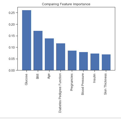
Glucose, followed by BMI and Age have the greatest importance among our features. This is most likely because of the separation glucose levels provide between being diagnosed with diabetes or not within our data set. Once again not really a surprise, given its the hallmark trait of the disease. However BMI and Age are both interesting features of importance.

The average confusion matrix for 4 fold cross validation is shown below.

Logistic Regression

Logistic regression relies on a linear equation passed to a function that returns an output of 0 or 1 such that it can be used for classification.

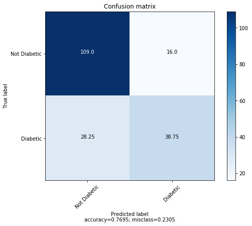
Logistic Regression accuracy: 76.95%.

The tune hyper parameter was: C = 0.03359818286283781

The average confusion matrix for 4 fold cross validation is shown below.

Support Vector Machine (SVM)

Initially we applied the dataset to a Perceptron Classifier in order to determine whether or not the data was linearly separable. By using the Perceptron Classifier, we discovered that the data was in fact linearly separable and the SVM may perform well on our data. SVM focuses on creating a hyperplane that separates two classes of data points.

The average confusion matrix for 4 fold cross validation is shown below.

The tune hyper parameter was: C= 0.1

Support Vector Machine accuracy: 76.43%

Conclusion

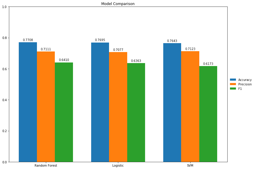Comparing the three best performing models, Random Forest had the highest accuracy at 77.1, SVM and Random Forest were incredibly close in precision at 71.23 and 71.11 respectively, and Random Forest had the highest F-1 score at 64.10. Additionally, Random Forest resulted in the least number of false negatives. This is extremely important in medical prognosis as we do not diagnose a patient as not having diabetes when they actually do, because that could put their life in danger and lead to other health problems.

Random Forest was especially interesting as it also showed that glucose was the most important feature in diagnosing diabetes, which is fitting, but also revealed that the Diabetes Pedigree was not important as other features such as age and BMI. This suggests that environmental factors such as glucose level rather than the genetic factors described by the Diabetes Pedigree are more strongly correlated with a diagnosis of Diabetes.

Random Forest likely performed the best due to the unbalanced nature of the dataset; it was less affected by this imbalance than the other algorithms. It also tends to do better classifying when there are only a few key features. Overall, the three best models either met or exceeded prediction expectations of 70% accuracy.

One thing to consider for future work in this field is the distribution of the dataset; most of the outcomes were no diabetes instead of a more even split. We speculate that with a more evenly distributed dataset, perhaps a data set that included a more diverse people outside of the pima indians, we would have had more accurate results.

References:

1. Balkau, Beverley, et al. “Predicting diabetes: clinical, biological, and genetic approaches: data from the Epidemiological Study on the Insulin Resistance Syndrome (DESIR).” Diabetes care 31.10 (2008): 2056-2061.
2. Kandhasamy, J. Pradeep, and S. Balamurali. “Performance analysis of classifier models to predict diabetes mellitus.” Procedia Computer Science 47 (2015): 45-51.
3. Mani, Subramani, et al. “Type 2 diabetes risk forecasting from EMR data using machine learning.” AMIA annual symposium proceedings. Vol. 2012. American Medical Informatics Association, 2012.
4. Zheng, Yan, Sylvia H. Ley, and Frank B. Hu. “Global etiology and epidemiology of type 2 diabetes mellitus and its complications.” Nature Reviews Endocrinology 14.2 (2018): 88. Zou, Quan, et al. “Predicting diabetes mellitus with machine learning techniques.” Frontiers in genetics 9 (2018).